Study 11: Revisiting the Devil's Card Game (no-code)
Considering risk of ruin, compounding, & volatility clustering
The Devil’s Card Game is a thought experiment that makes us decide how early to take profits or cut losses during an uncertain game. It’s a fun game for investors.
It has a key flaw though - at each stage of the game, all probabilities are known. This is totally different from markets, where we have to guess about future probabilities.
Why Consider This Game?
A popular solution is incorrect when we consider compounding; I want to show this is the case through simulation.
It involves similar tradeoffs to holding US stocks - positive long-term gains with larger short-term potential pain.
We can use it to visualize the tradeoffs involved in cutting losses.
Note on risk - bigger drawdowns need even bigger rebounds to recover all losses.
Once a position falls 20%, it needs to rise 25% to fully reverse.
Once it falls 33.3%, it needs a 50% rise to fully reverse.
The plot below shows ratio of the “gain” (g) we need for a given “drawdown” (d) for our capital to get back to its initial value. Notice, [g/d] is always tilted above 1, and it worsens exponentially. It adds a convex risk.
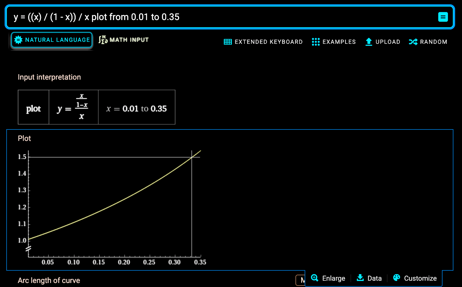
The equation comes from an example where we start with $1.
After a 3% drawdown (d) we have (1 - d) left. We need to grow it so (1 - d)*(1 + g) > $1.
(1 - d) * (1 + g) > 1
g = d / (1 - d)
ratio = g / d = (d / (1 - d) ) / d
Game Description
Imagine a bag that has 11 cards. 10 of them say “2”, and they multiply your money by 2 if you get one of them. Another card says “1/2048”, and divides your invested wealth by 2048 [causing a 99.95% drop] if you get it; this is known as the Devil’s card.
PS: Want to code this yourself? Check out the code in this post!
Before drawing any cards, we shake the bag up to shuffle them. Then, we pull a card one at a time from the bag without replacement. Once we start drawing cards, we can stop anytime, whether on card 1, or on card 11 (the last card).
Our initial capital is $1. We could stop at 3 cards. If we draw [2, 2, 2], we end up with 1*[(2)^3] = $8.
The longer we wait to stop drawing cards, the higher the odds of getting the Devil’s card. The first time we draw a card we have a 1/11 chance in getting the Devil’s card. The second time we draw, we have a 1/10 chance (assuming we didn’t draw it already). On the other hand, staying in longer also unlocks more chances to double your wealth and get higher overall returns.
Keep in mind, if we get the Devil’s card before we stop, we should play until the end. Since we already have the one bad card, we know the rest of the cards are all “2” cards, which help us and multiply our wealth. Obviously, we should use those cards. By playing all of them, our wealth ends at 1*[(2)^10]*[(1/2048)^1] = $0.5, a 50% drop relative to our $1 starting capital.
This makes the game very unrealistic. Sometimes, we know that the rest of the cards are all “2” cards. But in markets, we never have scenarios where we know all future outcomes will be good [+EV].
Flawed Approaches for Selecting a Stopping Point
One way to select a stopping point is is to try each one and look at the average return that we expect to end with if we follow it. The problem with this is, it considers returns, but not the likely pain required to see those returns.
For example, using a stopping point of 10 cards gives us a 10/11 chance of losing & ending with a loss (a 50% drop), far too high.
A 50% drawdown is too steep for most traders.
Large drawdowns hurt returns by needlessly adding volatility drag (h/t Benn)
That said, let’s show the expected return approach.
Focusing on Expected Returns
Suppose our stopping point is card 2 (no more cards after the second card). There are 11 potential sequences of cards we might draw from; only two of them could make us pull the Devil’s card before stopping: [(1/2048), 2, 2, 2, 2, 2, 2, 2, 2, 2, 2], and [2, (1/2048), 2, 2, 2, 2, 2, 2, 2, 2, 2].
In both of those cases, we would hit the Devil’s card before stopping, so we would play all the cards and end with a 50% loss. In the other 9 scenarios, we never hit the Devil’s card. We stop after [2, 2], so our end return is (1*[(2)^2]) - 1 = 300%.
So when x=2 (stop=2):
Probability of loss: (x/11) = 2/11. return of loss: -50%
Probability of win: [1 - (x/11)] = 9/11, return of win: (1*2^x) - 1 = 300%
Expected return = (p_loss)*(return_loss) + (p_win)*(return_win)
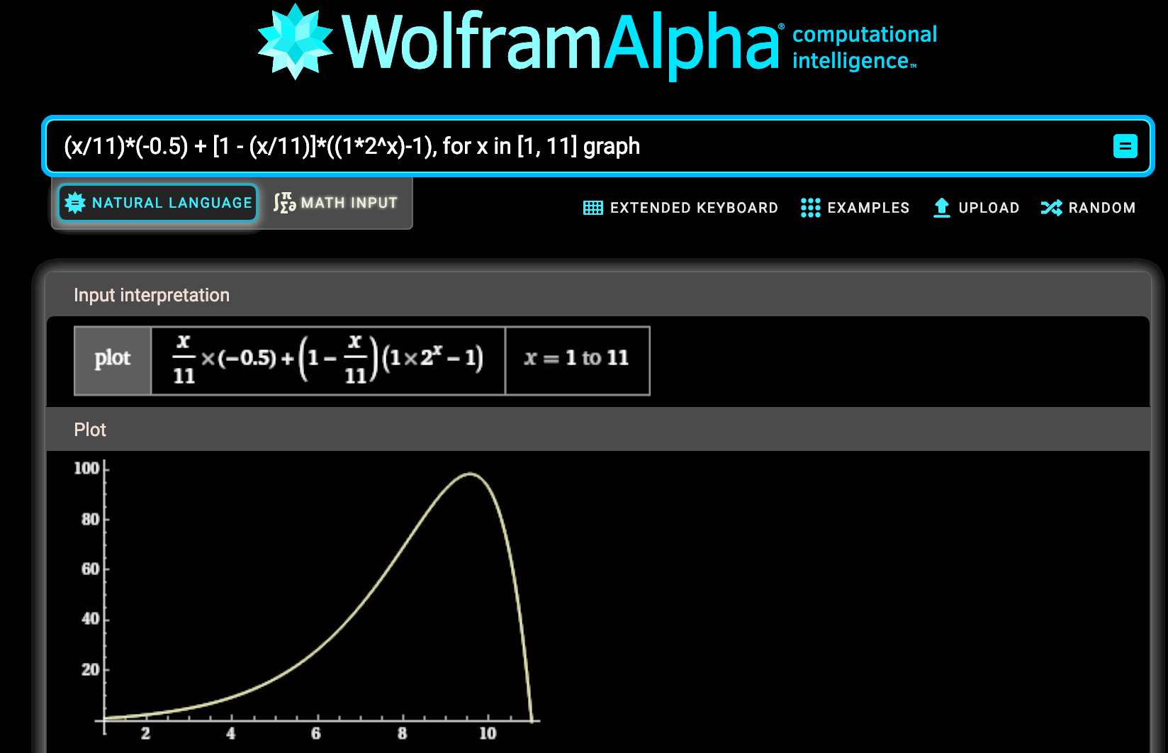
Expected return if stopping after card x = (x/11)*(-0.5) + [1 - (x/11)]*((1*2^x)-1)
We can graph this equation in WolframAlpha; it shows a peak expected return occurring at a stop point of around 9.5583 cards, which is closest to 10 cards; way too risky.
Focusing on Expected Returns vs Probability of a Bad Outcome
We can improve things a bit by looking at the ratio between expected return, and the probability of a bad outcome, like a loss [50% drop in capital in this case]. To do this, we can divide the original equation, by the probability of a loss (x/11), then find the max.
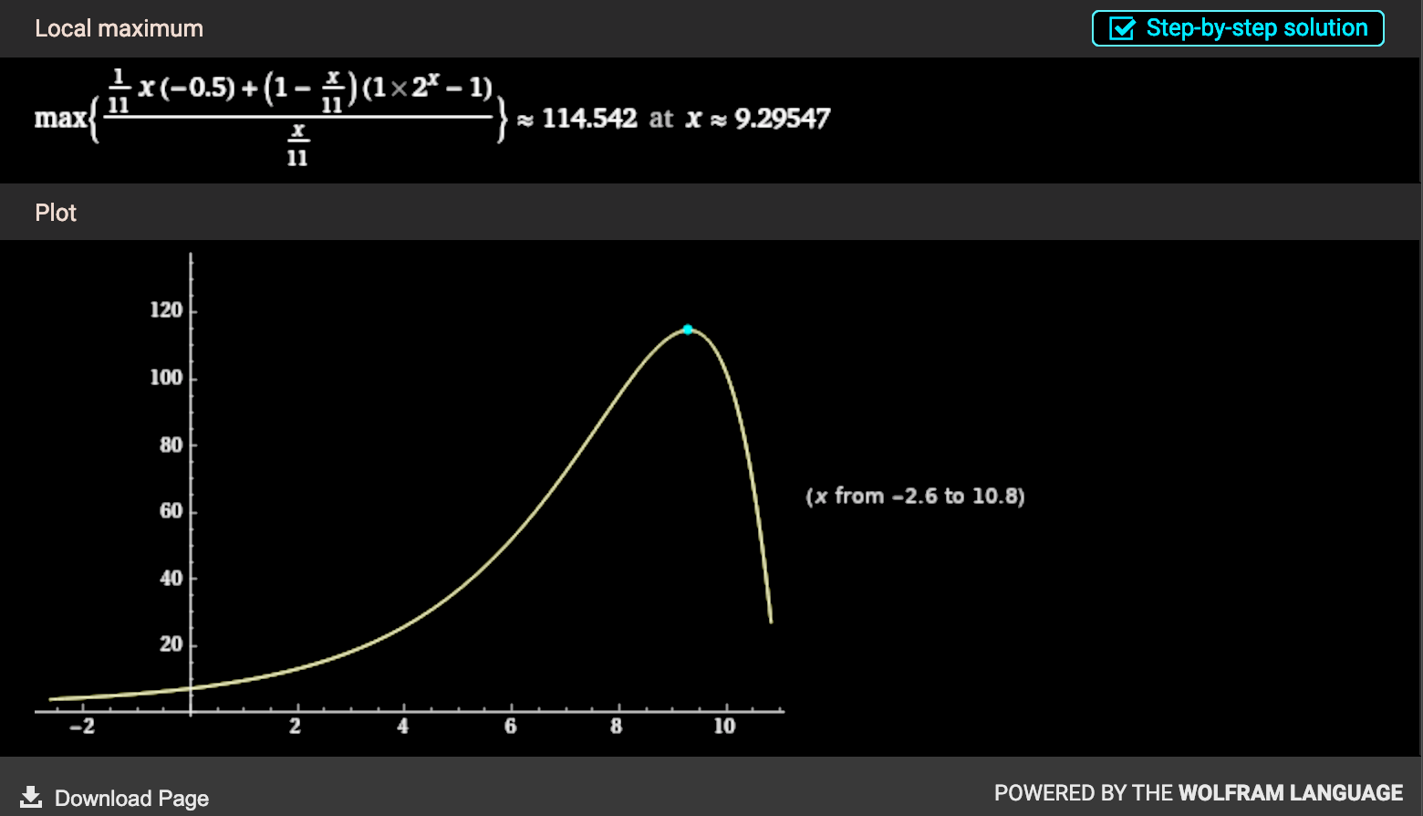
This is slightly more conservative than the first method, but it is still flawed.
In this case, it’s around 9.29547, which rounds to 9; slightly more conservative than the first equation, but still way too high.
Plus, the ratio is comparing a % return with a % probability, which is not necessarily logical [not apples-to-apples]. The former is unbounded while the latter is bounded.
Ratio of Ranks (Expected Return vs Probability of a Bad Outcome)
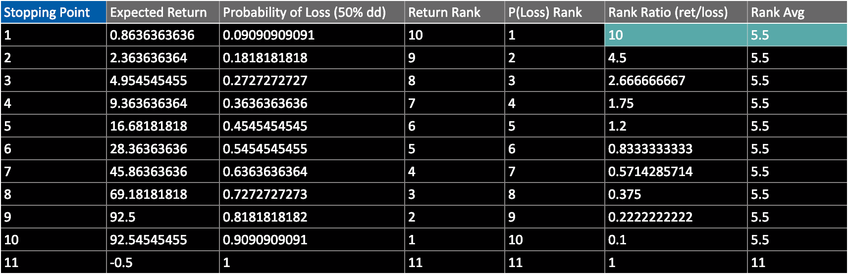
Another approach involves looking at each stopping point, and ranking the return it delivers among all our other potential choices for a stopping point. We can also rank the probability of a bad outcome for that stopping point. Now we have two ranks, and we can find the ratio between them, or the average of them. We do this for all stopping points and see which looks the best.
But using this method, we see that a stopping point of 1 has the highest ratio of ranks, and average rank. But this is likely too cautious (we are barely playing)!
Three Advantages of Using Realistic Simulation Instead
By simulating streaks of bets, we consider the messy realities of trading.
1: Compounding will exacerbate drawdowns
In a streak of bets, our overall max drawdown might exceed the per-bet max.
Imagine a coin with 90% odds of tails & 10% odds of heads. Tails gives us a 3% loss & heads gives us a 27% gain. The per-flip max drawdown is 3%. Expected return per flip is 0% ([0.90]*[-0.03] + [0.10]*[0.27] = 0).
But we have a 90% loss rate, so in the short term, we’ll likely have consecutive losses of 3%, leading to a total max drawdown well above 3%.
2: Returns come at a price (bad timing & paths), and should be compared to it
Suppose we lose 90% of the time.
If our losses all occur in the beginning, our portfolio will have a big initial drawdown.
If our losses are more evenly spread throughout the session of betting, our drawdowns will be smaller.
When we bet on a streak of games, we risk having unfortunate timing. If losses happen in clusters, we see bigger max drawdowns.
So if we are assessing a particular streak, we must consider the end return, *and* the max drawdown we went through to get that return (whether favorable or not). This is how we consider the impact of timing luck (autocorrelated losses).
3: Odds aren’t static - sudden pain increases odds of more [see “Cockroach Theory”]
In markets, volatility is often correlated with itself. A sudden increase in volatility is more likely to be followed by more volatility, not less. So events (like a vol spike) that happen now can change the odds of future events of interest.
A simulated approach can incorporate this. We can change the game design so that:
once a Devil’s card is hit, remaining cards have higher variance but same EV, or
once a Devil’s card is hit, remaining cards have higher variance and lower EV
How to Simulate the Game Realistically
For each stopping point, we simulate a large number (~4000) of trials.
Each trial corresponds to one day. That day, we walk to the casino to play the Devil’s Card Game repeatedly (40 times), using the same stopping point. Then, we leave.
The wealth we had at the end of our first game is invested into the second game, and so on. If we lose game 1, our wealth is 0.5 (50% below initial). Now the next time we draw a “2”, our wealth doubles from 0.5, to 1.
By looking at a streak of games, we consider compounding & timing luck.
We can use this to test the default style of the game, and a modified version. In the modified version, we assume that reward/risk in markets gets worse once a sudden shock happens. So once we hit a Devil’s card, the remaining cards are switched out with coins that have an expected value of “1” [0% return], not “2”, when drawn & flipped. We are committed to playing them, once the devil card is hit.
We can do this by building the coin to have a 50% chance of showing 1.99995, and a 50% chance of showing (1 / [10*2048]).
Here’s how we’ll measure and compare results. For each stopping point, we’ll look at the 20th, 50th, and 80th percentiles of returns, drawdowns, and pain-adjusted gains (returns minus drawdowns) experienced.
I applied a scaling factor to positive returns, because after 40 games they often became huge and hard to visually compare with drawdowns. To account for this, I tested various scaling factors so the charts are easier to see.
This applies to all trials, so it doesn’t change the relative performance of different stopping point selections.
I ended up looking at return^(1/60) to scale back big returns like 8.3 (830%, which scales back to 103%, not far from the biggest potential max drawdown)
Results - Devil’s Card Game (Standard Style)
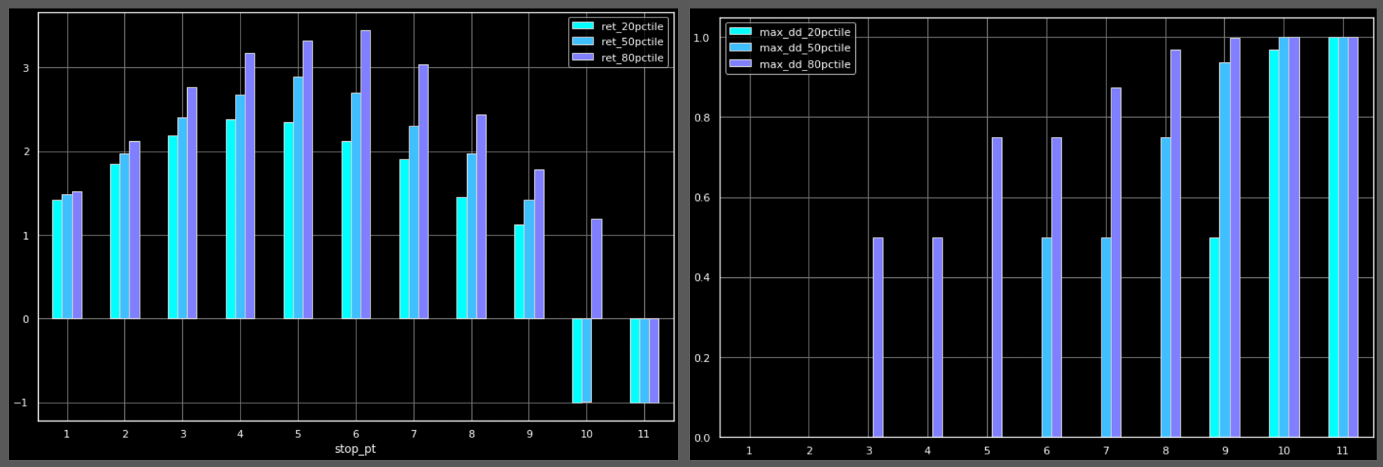
First we consider returns (left chart) & drawdowns (right chart). As we can see, median returns actually peak when we stop playing beyond 5 cards.
This differs from the results of this post, part of an interesting thread written by 10-k Diver about this game (it inspired this study!).
That post argued that the ideal stopping point might be 6 cards, but it had some key assumptions & flaws.
Assumed 50% of net worth is invested
Assumed starting capital is always 1
Ignored drawdowns suffered in order to get returns
What’s the takeaway? When assessing a single strategy or asset class, we should never start with assuming what % net worth we invest in it or what capital we have.
The first step should be to look at the average returns and drawdowns. If the pain-adjusted gains look good, we consider putting capital in play.
How much we bet (% net worth) depends on our acceptable % drawdown, vs the % drawdown of the strategy.
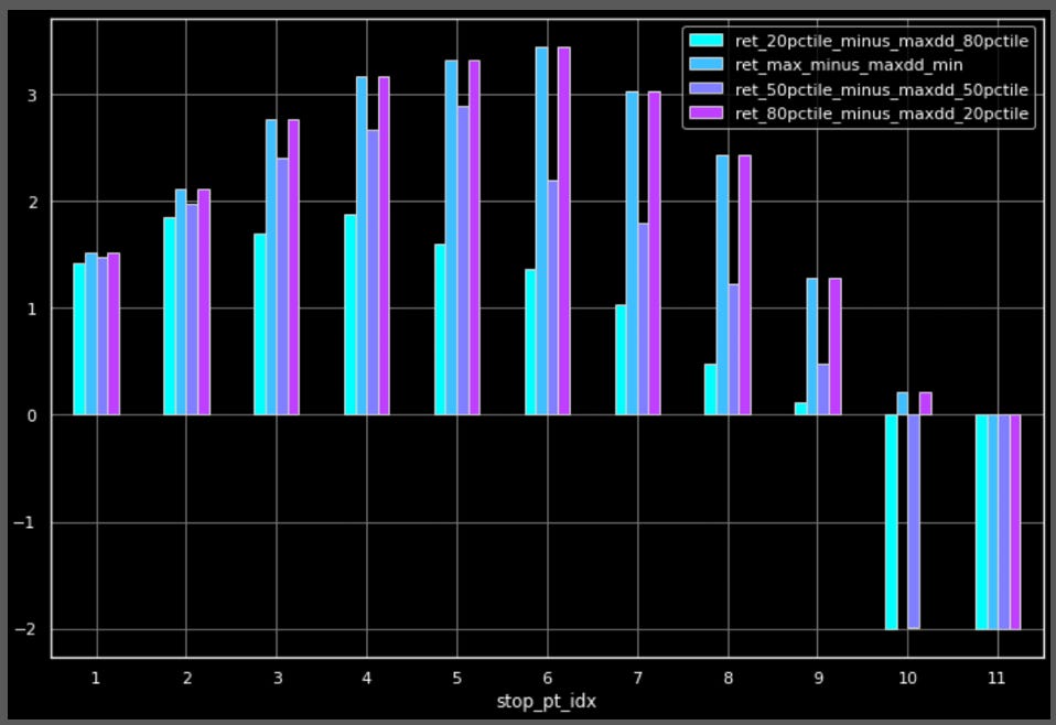
Finally, we’ll look at pain-adjusted returns to see what stopping point has the highest reward/risk ratio. As you can see, the median pain-adjusted return peaks at 5 as well.

Results - Devil’s Card Game (Modified, with Dynamic Odds)
Surprisingly, results were nearly identical to the default settings. I suspect this is because the game only changes when a Devil’s card is hit, which is rare by design, the long-term expectation of the modified game is probably similar to the original, and I used so many trials that the "true averages” got to play out.
The left chart has returns, and the right chart has drawdowns. The left chart looks different because I also plotted the “best” and “worst” return, and drawdown, so there are more bars. Aside from that, the charts are very similar to the results of the default game. The median return peaks at 5.
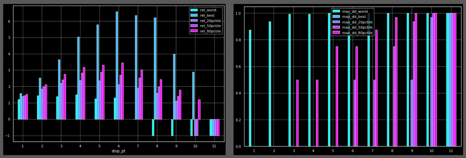
Now we’ll look at pain-adjusted returns to see what stopping point has the highest reward/risk ratio. As you can see, the median pain-adjusted return peaks at 5 as well. Adding vol clustering, at least the way I tried, didn’t have much of an impact.
Wrapping Up
When you consider compounding, the ideal stopping point (for max pain/gain) is different than most people think (and argued in a popular thread)
This game is a poor proxy for markets because we know our odds and potential payoffs at every stage of betting, and in advance. This is completely unrealistic for traders.
The risk of big drops is a valid similarity between this game and markets.
Maximizing utility should focus on returns & drawdowns of the asset or strategy in question, first. It shouldn’t start by assuming things about our net worth and nominal amount of capital.
And that’s it folks! Hope this inspired some new ideas and taught you a few python tricks. Cheers!