Study 10: Divergences Between Implied Volatility & Underlying Returns (no-code)
Can we learn about the future by comparing changes in VIX and SPY?

Some traders compare the recent return in SPY with the change in its option market’s expectations of future volatility (the VIX index).
This study tests this variable in depth, comparing it with future variables of interest like returns, risk-adjusted returns (per-drawdown), future volatility (GKYZ style), and changes in future volatility.
The Theory
High volatility usually occurs when the underlying drops.
If the option market’s expectations of future volatility become elevated, this implies the market is getting more concerned about future drops.
In a simple world where stock & option traders have similar information, we would expect stock traders to get spooked about the underlying fairly soon after the options market.
The underlying price should probably drop if the market believes a future period of high volatility & potential pullback is likely (SPY drops should accompany VIX rises).
If that isn’t the case, maybe there are greater odds of future return or volatility in the underlying looking different than they normally do.
PS: want to code this yourself? Check it out here!
Issue with VIX
The VIX index isn’t tradable, and some of its movements stem from the quirks of the formula that calculates it.
It considers volatility over the next 30 calendar days (including today). It does not consider weekend days as a source of potential volatility (as Benn Eifert discussed here).
On Friday, the next 29 days include 5 weekend periods, while on Thursday, the next 29 days include only 4 weekend periods. The Friday calculation has a higher fraction of days that get ignored, so the VIX level tends to be lower that day.
This is a non-tradable artifact of the math underlying the VIX. Instruments that reference the VIX all consider this effect already (markets are pretty smart), so we can’t purely bet on it; it just complicates our analysis.
Alternative: VOLI
VOLI, an index created by Nations, is free of those quirks and is a simpler measure of expectations of future volatility.
“VOLI is comprised of the first in-the-money and first out-of-the-money call and put options for the four weekly expirations bracketing the moment precisely 30 days in the future. These 16 option components are interpolated to generate a mathematically robust, closed-form measure of at-the-money, precisely 30 days to expiration, implied volatility.” (see Nations’ materials on VOLI)
I multiply it by (1/100) since my calculations display 20% as 0.20, while VOLI shows it as 20.
Creating Variables
Using daily data from June 2013 to March 2022, we can calculate the recent return in SPY and subtract the recent level-level change in VOLI (taking today’s VOLI value and subtracting the VOLI value from Z days ago).
Then we can compare that measure (aka “x”) with several future variables of interest: returns, drawdown-adjusted returns, GKYZ volatility, and changes in GKYZ volatility (for example - the difference between trailing 20-day GKYZ vol today, vs 20 days from now).
Those variables can relate to one asset, like DBO (an oil ETF), or be cross-asset, like the spread between future returns in EEM and VT.
We need several parameters to build these variables, like how far to look ahead (window_y), what asset or pair of assets we hope to predict (asset_y), and what sub-region or quantile of x to focus on (num_quant - optional). We can look at a range of values for all of these parameters and test all unique combinations of them. Itertools allows us to generate all of those combinations.
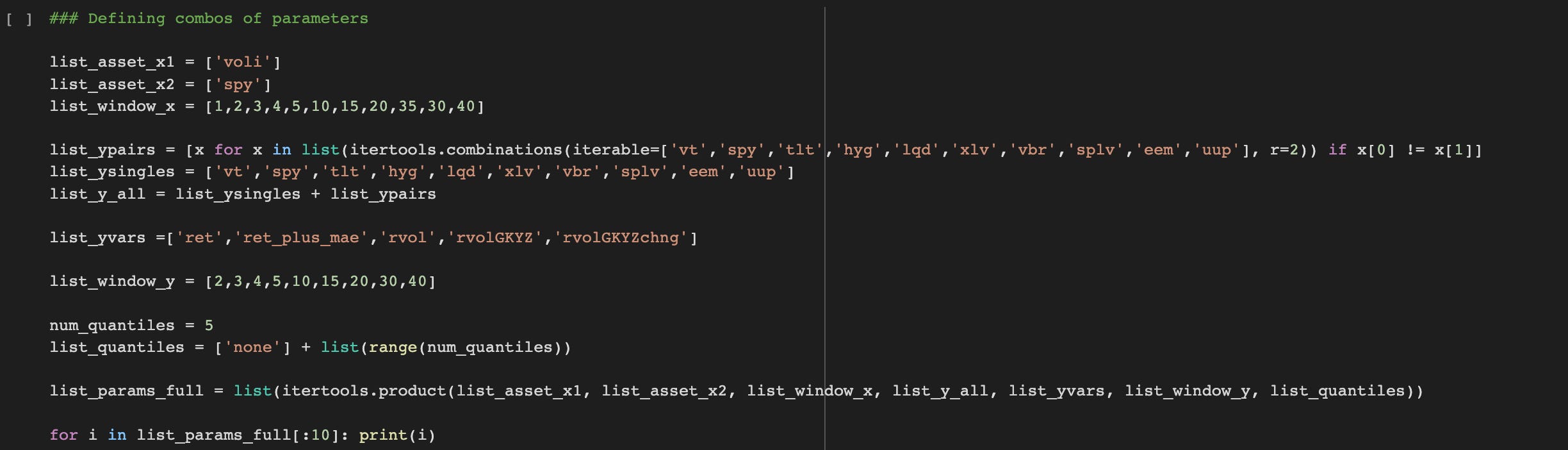
Each combination will be a tuple, like this:
('voli', 'spy', 40, ('eem', 'uup'), 'rvolGKYZchng', 30, 3)
Which corresponds to these parameters:
asset_x1, asset_x2, window_x, asset_y, var_y, window_y, num_quant
Assessing Predictive Value
Once we have our x and Y variables, we can use simple linear regressions to identify if a general relationship exists between them.
We can also zoom into our x variable and see if a particular region of it has signal.
We can compare the distribution of Y in the entire sample with the distribution of Y on days when x is in a particular quantile (like quantile 1 of 5 [the bottom 20%]).
We’d like to see a big difference between the distributions, with a KS statistic of close to 1 and with a fairly large difference between the medians (50th percentile) of those distributions.
I like to look at each distribution’s 20th and 80th percentile values out of curiosity as well, preferring to see a shift in all percentiles in the same direction.
Regression Results
After an exhaustive search, I only found one regression with a non-zero R squared value.
Here, x is ([SPY’s 15-day return] - [VOLI’s change from 15 days ago]), and Y is future volatility over the next 20 days for VBR, an ETF that bets on small-cap value stocks.
That regression suggests that lower values of x have a tendency to be associated with higher values of future volatility in VBR. What could cause values of x to be low?
SPY drops at same time that VOLI rises or barely moves
SPY moves up but VOLI rises much more
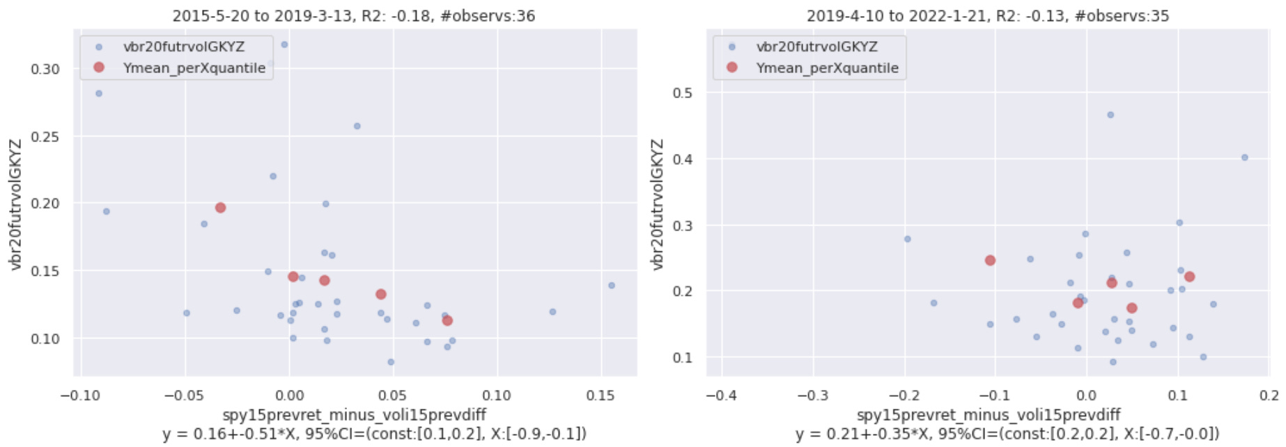
Since the R squared value is pretty low, with a magnitude below 0.2, this relationship is not very strong.
This suggests that looking at the spread between changes in SPY and VOLI doesn’t tell us much about the future. However, it’s possible that certain quantiles of that spread could have signal.
Quantile Results - Preview
Several quantiles were associated with our future variables looking different than they typically do.
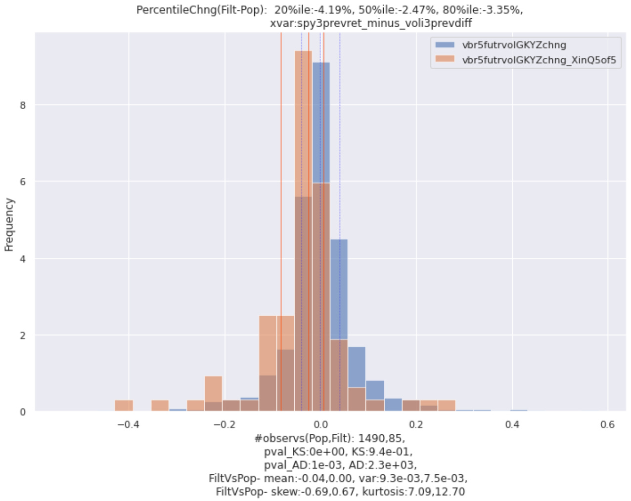
In the plot below, x is ([SPY’s 3-day return] - [VOLI’s change from 3 days ago]). Y is the future change in VBR’s trailing volatility ([VBR’s trailing volatility 5 days from now] - [VBR’s trailing volatility today]), where trailing volatility is computed with a 5-day lookback.
When x is fairly high (in quantile 5 of 5 [highest 20%]), future changes in VBR’s volatility tend to be more negative than they are in the overall sample.
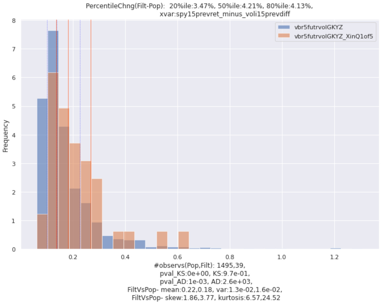
In the next plot, x is similar to the one above but uses a 15-day lookback. Y is the future volatility in VBR over the next 5 days (rather than the future *change* in volatility).
As our regression implied, when x is fairly low (in quantile 1 of 5 [lowest 20%]), VBR’s future volatility tends to be higher than it is in the overall sample.
To see more results, check out this post right here!
Closing Observations
It was easier to find signals relating to future volatility or future changes in volatility; no directional signals were found.
Low values of x (SPY return - VOLI change) are associated with higher levels of future volatility in VT and VBR. High values of x are associated with more negative changes in future volatility in VT and VBR.
Only one notable cross-asset relationship was found.
Overall, the spread between SPY and VOLI (or VIX) changes is unlikely to provide insight about the future unless we are checking to see if the spread falls into the lowest or highest historical quintile.
And that’s it folks! Hope this inspired some new ideas and taught you a few python tricks. Cheers!