Momentum vs Random Entries (no code)
Contrasting the returns, MAEs, and risk-adj returns for small-cap equities

Can a momentum-based strategy beat random entries in small-cap stocks?
Let’s explore this question by considering a long-only momentum strategy that is invested when momentum is strong (short-term trend > long-term trend) and flat otherwise. (PS: this post was inspired by this tweet from Darrin). In this case, we measure trends by looking at exponential moving averages.
For the sake of conservatism, this strategy will be optimized for a training portion and then tested in the most recent 40% of the dataset.
This problem was more of a puzzle than I initially expected, but we can break it down into these steps:
Define our universe of stocks to consider
For each, find the ideal momentum strategy based on the first 60% of our sample
Store the length of all the long trades in the strategy as a distribution. Do the same for the trade-free time periods.
Look at the probability of beginning a long trade (instead of a flat period)
Simulate a random entry system; use the probability above to flip a coin.
The coin tells us whether to draw from the distribution of long trades or flat trades. Then, we randomly select the trade length from that particular distribution. Repeat this until the total number of time increments spent long or flat exceeds the number of increments in our sample.
Simulate this 1000 times in total.
Then we can compare the performance of the momentum strategy and random entry strategy.
We’ll analyze the testing period (final 40% of our sample) by looking at rolling returns, rolling MAE (max adverse excursion), and rolling [return - MAE], which measures the difference between gain and pain. For those unfamiliar with MAE: if you buy Facebook stock at 100, it dips to 98, then rises to 105, your max pain (aka MAE) is (98/100) - 1 = -2%.
Defining the Universe
Ideally, we would construct our universe based on the information available at the start of the sample (about 10 years ago), however I currently lack the data needed to do that.
As an alternative, we can just filter based on the information available today. This unfortunately has survivor bias; we are only looking at securities that we know have been successful enough to stay listed up until the end of our sample.
On the other hand, this filter is very basic and hopefully won’t yield results that are that different from the ideal method.
I used a screen on finviz with the following requirements:
— Average volume above 1mil & share price above $5
— Securities that trade in the U.S.
— Market cap below $2bil & IPO date at least 10 years ago
Then I sorted the results based on their average volume, from highest to lowest, leading to the following results:
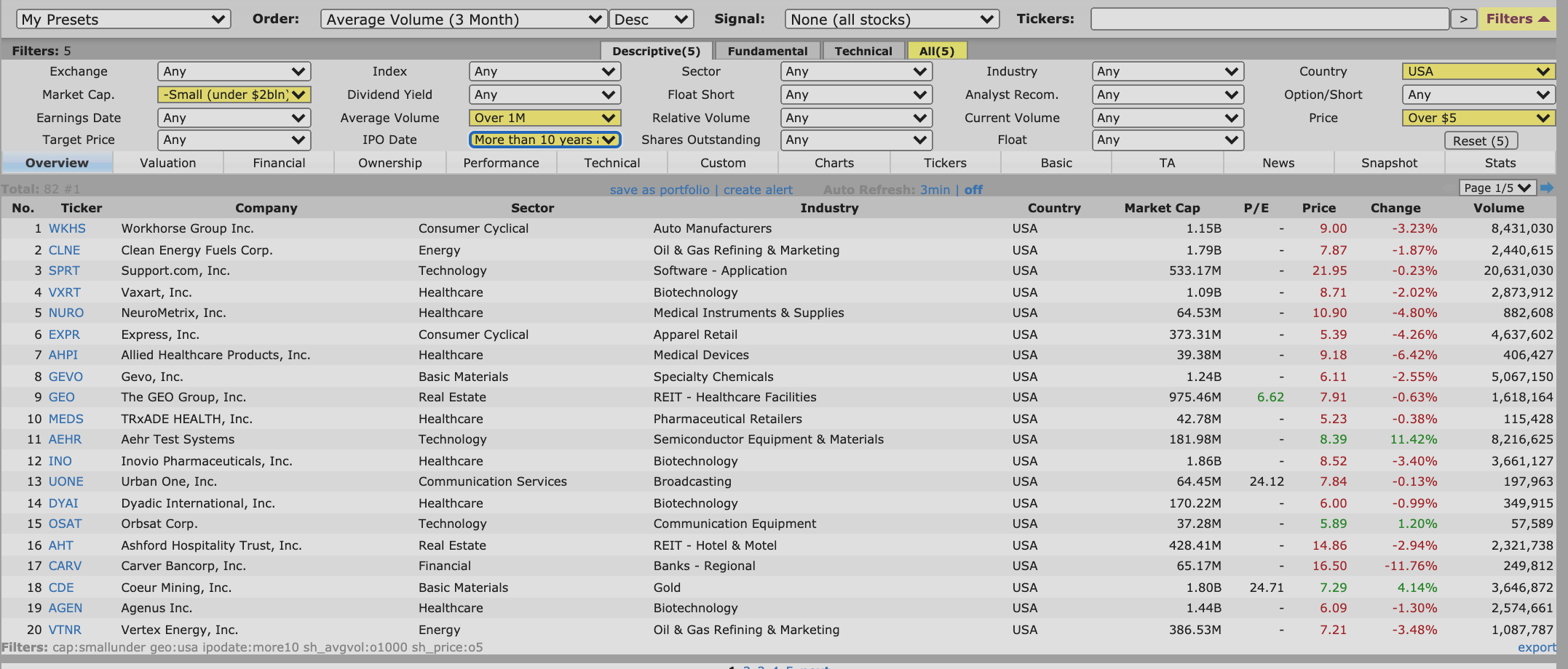
After sorting by average volume, I selected the first 20 securities with about 10 years of price history, and I also downloaded the price history for the iShares microcap ETF (IWC) as an additional security to test.
Viewing & Measuring Performance
To compare our momentum strategy with random entries, the first thing we need to do is generate the equity curve that results from trying the momentum strategy. This is shown in black below; it is optimized for the training portion, which ends once the black line crosses the horizontal axis. The rest of the lines show the equity curves of our 1000 attempts at using random entries during the sample instead.
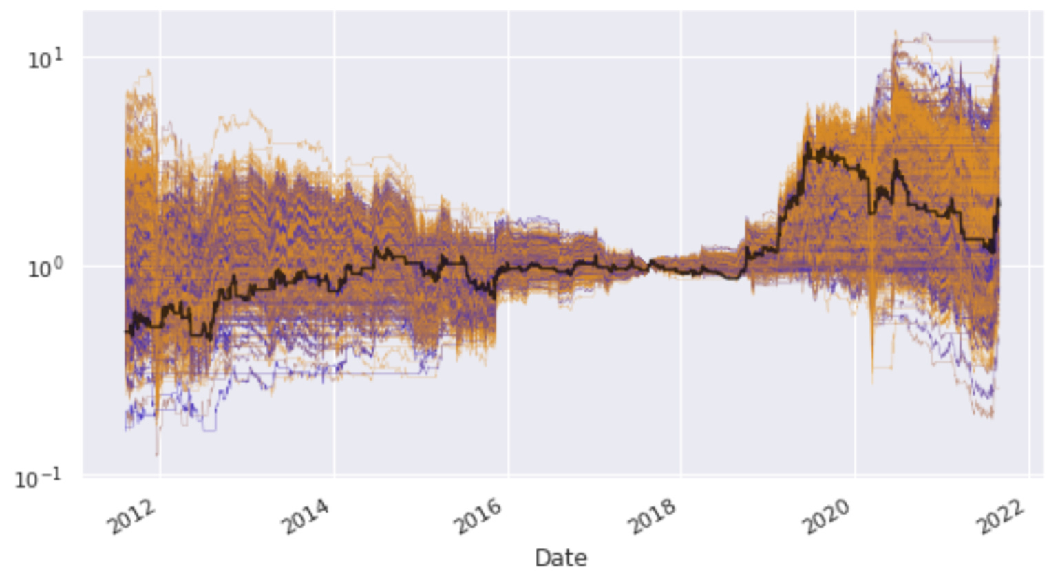
PS: Want to learn how to implement this in Python? This post has the full code!
Once we have our equity curves, we look at trailing performance metrics (like returns & MAE) in our testing portion. We need to remove overlapping measurements of these metrics so we don’t fool ourselves into thinking we have a larger number of unique data points than we really do.
Consider returns. First, we can find the momentum strategy’s trailing returns, remove overlapping readings, and then store them in a distribution. We want to compare it to the return distribution that comes from our random entry attempts.
We have 1000 equity curves that used random entries. We can find the trailing returns for each one, remove the overlapping readings, and then add those data points into our a list. This list stores the returns for all 1000 attempts at trading a particular security randomly. We can then plot it as a distribution and see how different it is from the distribution that came from trading the security using the momentum strategy.
The Kolmogorov–Smirnov statistic will help us see how different these distribution are. The closer the “KS” score is to 1, and the lower the related p-value is, the more different the two distributions being compared are from one another.
Check out the image below, which shows an example for the security CDE. This looks at trailing MAE (pain) rather than trailing returns. When MAE is more negative, trailing pain is higher.
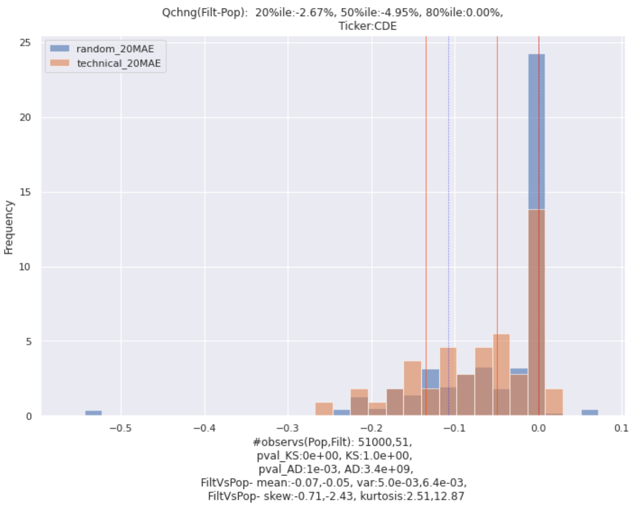
The orange distribution, aka “filt”, shows the trailing MAEs resulting from our momentum strategy. The blue distribution, aka “Pop” (short for population) shows the trailing MAEs for all 1000 uses of the random-entry strategy on this security.
I added vertical lines at the 20th, 50th, and 80th percentile values of these distributions so we can more clearly see the differences. The title of the plot summarizes the percent differences between the orange distribution’s vertical lines and the blue distribution’s vertical lines.
In this example, the momentum strategy’s median MAE (50th percentile) is 4.95% more negative than the random-entry strategy’s median MAE.
To summarize the overall difference between these distributions, I also calculate the average % change in quantile values. In this example it would be:
(-2.67% + -4.95% + 0%) * (1 / 3) = -2.54%
We will use a similar process for other trailing metrics like returns, and [returns - MAE]. Finally, we can store all of those results in a table. It should look like the one below.
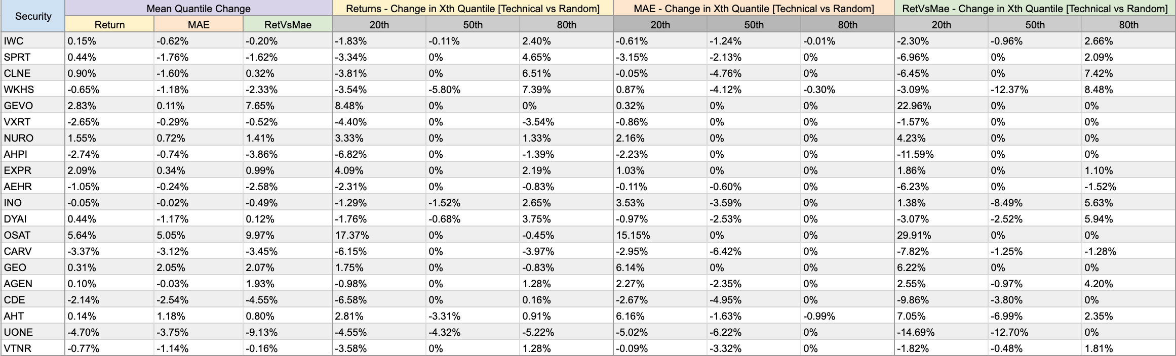
Results
By plotting the first four columns of this table, we can get a sense of the overall changes in these three performance metrics that we get when using momentum rather than random entries.
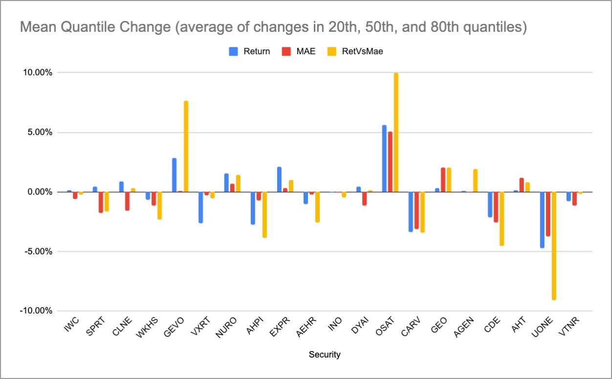
This shows the mean changes for each security, but if we average them together, we’ll see the average effect of the momentum strategy on our overall universe (all securities).
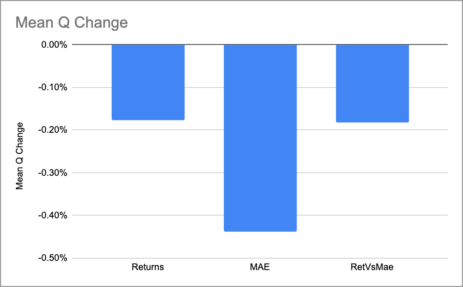
Overall, it seems like Darrin’s claim was valid. Trying to outperform a random-entry system in small-caps is difficult. This particular momentum strategy, which uses two different rolling averages, failed to do so. It led to worse returns, worse MAEs, and worse risk-adjusted returns than just randomly entering and exiting. (Of course, it’s perfectly possible that other price-action strategies could do quite well; I have been surprised many times.)
Keep in mind that slippage will affect our results. However, since I designed the random strategy to have a similar number of trades as the momentum strategy, this variable should end up having a similar impact on both strategies, so I chose to set it to 0. Luckily I have designed this as a custom parameter that you can tweak and experiment with: slippage as a % of 14-day trailing ATR.
Hope you enjoyed this experiment!
Until next time,
Mitch